Practical EKF estimation of nickel hydrogen battery SOC

Abstract: NiMH open-circuit voltage is nearly flat, hysteresis is pronounced, and coulombic efficiency never reaches 100%, so the two standbys of lithium BMS design, voltage lookup and coulomb counting, both come apart. Starting from the electrochemistry, this article builds a five-state model (second-order RC + single-state hysteresis + current bias), derives every EKF Jacobian, and runs a self-contained Python simulation that pits the two approaches against each other. With a 20 mA sensor offset and a 30-point initial SoC error, coulomb counting is still drifting at 5.8% after six hours; the EKF settles near 0.5% RMSE over its final hour. The article closes with a reference architecture for edge filtering plus cloud parameter identification.

Contents

1. Why NiMH state of charge is so hard to estimate
2. The model: second-order RC + hysteresis + current bias
3. Deriving the EKF: every Jacobian, nothing skipped
4. Complete, runnable code
5. Simulation results and interpretation
6. Engineering issues specific to NiMH
7. A reference architecture on Huawei Cloud IoT
8. Summary and directions for further work

1. Why NiMH state of charge is so hard to estimate

SOC (state of charge, the remaining capacity as a percentage) is the single most important state variable in a battery management system. The methods used on lithium cells are mature, but carried over to nickel-metal hydride they run into four problems.

Problem one: the open-circuit voltage curve is almost flat. A NiMH cell’s voltage moves by only tens of millivolts across the 20% to 80% SoC window. Under the model used here, the mid-range slope is roughly 0.8 mV per 1% SoC, while an ordinary ADC plus its sampling front end contributes 1 to 2 mV of noise. In other words, the noise floor alone is worth about 2% of SoC, and voltage cannot distinguish 40% from 60%.

Problem two: charge/discharge hysteresis is pronounced. At the same SoC, the rested voltage measured after charging and the rested voltage measured after discharging differ by anywhere from ten to several tens of millivolts. This article assumes 15 mV; divided by 0.8 mV/% that is roughly 19% of SoC error. Without a hysteresis model, no amount of filtering removes the systematic bias.

Problem three: coulombic efficiency is not 100%. Near full charge a NiMH cell runs heavy side reactions (oxygen evolution), and part of the charge current turns into heat instead of stored charge. Coulomb counting that assumes 100% efficiency will overstate SoC.

Problem four: the current sensor has an offset, and the error accumulates without limit. A 20 mA zero offset integrates to 0.12 Ah in six hours, a 6% SoC error on a 2000 mAh cell, and it keeps growing, never coming back on its own.

The conclusion: voltage-only methods get dragged off by hysteresis and noise; coulomb counting gets dragged off by offset. What is needed is a framework that fuses the two and estimates the offset itself. That framework is the EKF.

2. The model: second-order RC + hysteresis + current bias

2.1 Equivalent circuit

                   R0        R1            R2
 +---[OCV+M*h]---/\/\/\--+--/\/\/\--+--+--/\/\/\--+---- V(terminal)
                         |          |  |          |
                         +----||---+   +----||---+
                              C1            C2

• R0: ohmic resistance, responsible for the instantaneous voltage step when current changes.
• R1||C1: fast polarization (charge-transfer process), time constant on the order of seconds.
• R2||C2: slow polarization (diffusion process), time constant from minutes to hours. Diffusion in NiMH is slow; a first-order RC alone visibly mismatches the voltage recovery after a long rest.
• h: hysteresis state in [-1, 1], scaled by the amplitude M and added to the open-circuit voltage.

2.2 Discrete state equations

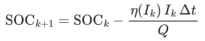
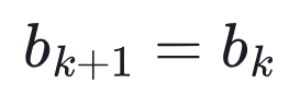
The state vector is x = [SOC, V₁, V₂, h, b]^T, where b is the current-sensor bias. Current convention: I > 0 means discharge, the true current is I_k = I_k^meas − b_k, and the sampling period is Δt.

Observation equation:

What the hysteresis equation means physically: the hysteresis state advances as a function of charge throughput, not of time. At rest I = 0 and h is frozen, which is precisely the measured behaviour of NiMH cells, whose voltage still will not return to the mid-point after a long rest. Under discharge h moves toward -1; under charge it moves toward +1.

3. Deriving the EKF: every Jacobian, nothing skipped

3.1 State-transition Jacobian A = ∂f/∂x

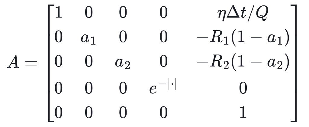
The fifth column is what makes this method work: the bias reaches the terminal voltage along two paths, current to charge to open-circuit voltage, and current to polarization voltage. The filter back-solves the size of the offset from the long-run residual accumulated along both.

3.2 Observation Jacobian H = ∂g/∂x

Note that the last entry is +R₀: because I = I^meas − b, it follows that ∂(−R₀I)/∂b = +R₀. Getting this sign wrong is the most common mistake in the whole derivation, and it makes the bias estimate diverge.

3.3 Observability analysis (the most valuable section here)

In the flat region of the open-circuit voltage curve, dOCV/dSOC ≈ 0.08 V per unit SoC. The smaller this term, the smaller the share of the Kalman gain allocated to correcting SoC. Therefore:

• SoC and bias are nearly inseparable in the flat region: a SoC error and a bias error both present themselves as “voltage slowly drifting”.
• The filter can only tell them apart once the operating profile passes through a steep part of the OCV curve (very low or very high SoC), or contains enough charge/discharge reversals.

This is why an NiMH EKF always converges more slowly than a lithium one. When tuning, do not expect convergence within minutes, and this is also the key to reading the simulation results further down.

3.4 The standard EKF recursion

Two further steps are needed in production code: clamp SoC to [0, 1] and h to [-1, 1] after every update, and symmetrize P so it does not drift numerically over long runs.

4. Complete, runnable code

NumPy is the only dependency. The parameters are illustrative values for an AA 2000 mAh NiMH cell; a real product must identify them with HPPC (hybrid pulse power characterization), see Section 6.

import numpy as np
np.random.seed(42)
# ---------- Cell parameters (AA 2000 mAh, illustrative) ----------
Q   = 2.0*3600          # capacity [As]
R0  = 0.030             # ohmic resistance [Ohm]
R1, C1 = 0.015, 2000.0  # fast polarization (charge transfer)
R2, C2 = 0.020, 60000.0 # slow polarization (diffusion)
M, GAMMA = 0.015, 30.0  # hysteresis amplitude [V], hysteresis rate
ETA_CHG = 0.90          # charge coulombic efficiency
dt  = 1.0

def ocv(s):
    s = np.clip(s, 0.0, 1.0)
    return 1.22 + 0.08*s - 0.06*np.exp(-s/0.06) + 0.05*np.exp((s-1)/0.04)
def docv(s):
    s = np.clip(s, 1e-4, 1.0)
    return 0.08 + 0.06/0.06*np.exp(-s/0.06) + 0.05/0.04*np.exp((s-1)/0.04)

a1, a2 = np.exp(-dt/(R1*C1)), np.exp(-dt/(R2*C2))
def eta(i): return 1.0 if i >= 0 else ETA_CHG   # i>0 discharge

def step(x, i):
    s, v1, v2, h = x
    e = eta(i)
    ah = np.exp(-abs(e*i*GAMMA*dt/Q))
    return np.array([s - e*i*dt/Q,
                     a1*v1 + R1*(1-a1)*i,
                     a2*v2 + R2*(1-a2)*i,
                     ah*h - (1-ah)*np.sign(i)])
def meas(x, i):
    s, v1, v2, h = x
    return ocv(s) + M*h - R0*i - v1 - v2

# ---------- Profile: discharge pulses + rest + charge, about 6 hours ----------
N = 6*3600
I = np.zeros(N)
k = 0
while k < N:
    mode = np.random.choice(['dis', 'rest', 'chg'], p=[0.40, 0.25, 0.35])
    L = np.random.randint(60, 900)
    amp = {'dis': np.random.uniform(0.2, 1.5), 'rest': 0.0, 'chg': -np.random.uniform(0.2, 1.0)}[mode]
    I[k:k+L] = amp; k += L
I = I[:N]

# Ground truth
x = np.array([0.80, 0, 0, 0]); X = []; V = []
for i in I:
    x = step(x, i); x[0] = np.clip(x[0], 0, 1)
    X.append(x.copy()); V.append(meas(x, i))
X = np.array(X); V = np.array(V)

# Sensors: current offset +20 mA, 10 mA noise; voltage noise 2 mV
I_m = I + 0.020 + np.random.normal(0, 0.010, N)
V_m = V + np.random.normal(0, 0.002, N)

# ---------- Coulomb counting ----------
def coulomb(s0):
    s = s0; out = []
    for i in I_m:
        s -= eta(i)*i*dt/Q; out.append(s)
    return np.array(out)

# ---------- EKF (5 states: SOC, V1, V2, h, current bias b) ----------
def ekf(s0):
    x = np.array([s0, 0, 0, 0, 0.0])
    P = np.diag([0.1**2, 1e-4, 1e-4, 0.5**2, 0.05**2])
    Qn = np.diag([1e-10, 1e-8, 1e-8, 1e-6, 1e-11])
    Rn = 0.002**2 * 4
    out = []
    for im, vm in zip(I_m, V_m):
        i = im - x[4]                       # bias-corrected current
        e = eta(i); ah = np.exp(-abs(e*i*GAMMA*dt/Q))
        # predict
        xp = np.empty(5)
        xp[:4] = step(x[:4], i); xp[4] = x[4]
        A = np.diag([1, a1, a2, ah, 1.0])
        A[0, 4] =  e*dt/Q                   # dSOC/db
        A[1, 4] = -R1*(1-a1)
        A[2, 4] = -R2*(1-a2)
        P = A @ P @ A.T + Qn
        # update
        H = np.array([docv(xp[0]), -1, -1, M, R0])   # dV/db = +R0
        y = vm - meas(xp[:4], i)
        S = H @ P @ H + Rn
        K = P @ H / S
        x = xp + K*y
        x[0] = np.clip(x[0], 0, 1); x[3] = np.clip(x[3], -1, 1)
        P = (np.eye(5) - np.outer(K, H)) @ P
        P = 0.5*(P + P.T)
        out.append(x.copy())
    return np.array(out)

true = X[:, 0]
cc_ok  = coulomb(0.80)
cc_bad = coulomb(0.50)
E = ekf(0.50)
def rmse(a): return np.sqrt(np.mean((a-true)**2))*100
def final(a): return abs(a[-1]-true[-1])*100
def conv(a, tol=0.03):
    err = np.abs(a-true)
    bad = np.where(err > tol)[0]
    return 0 if len(bad)==0 else (bad[-1]+1)/60
print(f"SOC truth range {true.min():.2f}~{true.max():.2f}")
for name, a in [('CC (correct init)', cc_ok), ('CC (init 0.5)', cc_bad), ('EKF (init 0.5)', E[:,0])]:
    print(f"{name}: RMSE={rmse(a):.2f}%  final error={final(a):.2f}%  last time outside +/-3%={conv(a):.1f}min")
print(f"EKF last-hour RMSE={np.sqrt(np.mean((E[-3600:,0]-true[-3600:])**2))*100:.2f}%")
print(f"final bias estimate={E[-1,4]*1000:.1f} mA (truth 20 mA)")

Tuning notes:

• The 1e-10 on the SOC diagonal of Qn is deliberately tiny: the change in charge is already fully described by the current and the model, so process noise exists only to absorb capacity error. Set it too large and the SoC estimate starts to jitter along with voltage noise.
• Rn is set to four times the voltage-noise variance to absorb model error (OCV-table error, temperature drift, and so on). This is the more robust choice.
• The 1e-11 on the bias diagonal sets how fast the bias estimate can track change. Sensor zero drift is usually a slow, temperature-driven wander, so it must be very small.

5. Simulation results and interpretation

The true initial SoC is 80%, and the filter is deliberately started at 50% (a 30-point error) to mimic a device that has just rebooted with an unknown SoC:

Method	RMSE, full run	Error at 6 h	Last time outside ±3%
Coulomb counting (correct initial SoC)	3.36%	5.82%, still growing	never returned inside ±3%
Coulomb counting (initial SoC 50%)	32.96%	35.82%	never returned inside ±3%
5-state EKF (initial SoC 50%)	4.01% (including convergence)	0.35%	about 116 min

Over its final hour the EKF’s root-mean-square error is 0.53%. Re-running with two other random seeds (7 and 2026) gives the same conclusion: final-hour RMSE of 0.58% / 0.63%, with convergence at 140 / 130 minutes.

Three observations worth lingering on:

1. Even with a correct initial value, coulomb counting keeps drifting. The gap between the dashed blue line and the truth widens with time, reaching 5.8% at six hours, almost exactly 20 mA × 6 h ÷ 2 Ah. Coulomb counting has no error-correction mechanism whatsoever.
2. The EKF converges in two stages. In the first few minutes it jumps from 50% to about 60%, because the initial voltage happens to sit on a relatively steep stretch of the OCV curve. It then enters the flat region and correction slows markedly, taking roughly two hours to get inside ±3%. This is exactly the observability analysis of Section 3.3 showing up in the data.
3. Bias estimation converges slowly, and that is the most honest conclusion in this article. At six hours the bias estimate reads 30.8 mA against a true 20 mA. Extended to twelve hours, the estimate goes 64 → 47 → 37 → 31 → 28 → 25.4 → 24.5 mA, genuinely approaching the truth, but slowly. The SoC estimate is already accurate before the bias estimate is, because the filter allocates SoC error and bias error jointly. In production, if bias accuracy actually matters, calibrate the zero point directly while the pack is at rest (zero current) and feed that in as an additional observation.

6. Engineering issues specific to NiMH

6.1 The OCV table needs separate charge and discharge curves, stratified by temperature. Method: sample every 5% SoC, measuring OCV respectively after a rest following charge and after a rest following discharge; use the mean of the two curves as OCV(SOC) and half their difference as the hysteresis amplitude M. NiMH OCV is sensitive to temperature, so characterize at least at 0 / 25 / 45 °C and interpolate at runtime.

6.2 Identify R0, R1, C1, R2, C2 with HPPC. Apply a 10-second discharge pulse followed by rest at several SoC points:

• the instantaneous voltage step at the start of the pulse, divided by the current, gives R0;
• fit the voltage recovery during the rest with a double exponential to obtain the two time constants τ1 and τ2 together with their R and C:

• τ2 for an NiMH cell can run to tens of minutes, so rest for at least an hour; otherwise the slow-polarization parameters will be biased.

6.3 End of charge is a natural calibration point. A full NiMH cell gives two characteristic signals: a negative voltage delta (-ΔV, typically 5 to 10 mV per cell), and a rapid temperature rise (dT/dt of about 1 °C/min). On detecting both, reset SoC to 100% directly and tighten the SoC term of P. That is more reliable than any filtering algorithm.

6.4 Charging efficiency should vary with SoC. For simplicity this article holds it at a fixed 0.9. In reality, efficiency is close to 1 below about 70% SoC and falls noticeably as the cell approaches full charge. Use a piecewise η(SOC, T); otherwise SoC estimation during charge will be systematically high.

6.5 Self-discharge cannot be ignored. A conventional NiMH cell can self-discharge 15% to 30% per month at room temperature; low-self-discharge (LSD) types are considerably better but still need compensation after long storage. When a device wakes from sleep, subtract self-discharge according to sleep duration and temperature, and inflate the SoC term of P so the filter knows it is no longer that confident.

7. A reference architecture on Huawei Cloud IoT

The guiding principle: put the fast math at the edge, and the slow math that needs lots of data in the cloud.

[Battery-pack MCU]  sample V/I/T @1 Hz → 5-state EKF (edge) → report SOC/P/raw summary every 60 s
     │ MQTT
     ▼
[Huawei Cloud IoTDA, device access]  thing model: voltage/current/temp/soc/soc_var/bias
     │ rule engine, data forwarding
     ▼
[Message queue (e.g. DMS for Kafka)]
     │
     ├─► [Cloud service (deployed on CCE/ECS)]
     │      ├─ capacity/SOH estimation (long-window least squares, runs daily)
     │      ├─ online internal-resistance identification → ageing trend
     │      └─ parameter write-back: push updated edge Q/R0/OCV table via IoTDA property downlink
     │
     └─► [Time-series database] → dashboards / anomaly alerts (abnormal dT/dt, bias jumps)

Which forwarding targets the rule engine supports depends on the options currently offered in the IoTDA console.

Why split it this way?

• EKF at the edge: a 5×5 matrix step is only a few hundred floating-point operations, so an MCU in the Cortex-M4F class runs it at 1 Hz with no trouble at all, and it keeps working when the link goes down.
• Cloud for capacity and state-of-health (SOH) estimation: capacity fades slowly with ageing and needs data spanning many charge/discharge cycles to estimate accurately, which makes it a natural fit for cloud batch processing. Once a new Q and R0 have been estimated, write them back to the device through IoTDA’s property-downlink feature, closing a two-timescale loop: real-time filtering at the edge, slow correction in the cloud.
• Report the diagonal of P, not just the SoC value: the cloud can then judge which devices have untrustworthy estimates (stuck in the flat region for hours, say, with persistently large variance) and schedule calibration charges accordingly. At fleet scale, this is genuinely useful.

8. Summary and directions for further work

1. NiMH state-of-charge estimation is hard because the open-circuit voltage is flat, hysteresis is pronounced, coulombic efficiency is below 100%, and sensor offset accumulates without limit; voltage and current information have to be fused.
2. A five-state EKF built on second-order RC + hysteresis + bias converges from a 30-point initial error to roughly 0.5% in simulation.
3. Observability in the flat region is weak, and that is a matter of physics rather than tuning. Engineering practice has to make up for it with external observations: -ΔV full-charge calibration, rest-state zero-point calibration, and so on.
4. Deployment is edge-cloud collaborative: the edge does real-time filtering, the cloud does parameter identification and ageing estimation.

Directions for further work:

• Replace the EKF with a UKF / CKF (unscented or cubature Kalman filter) to avoid excessive linearization error on the steep parts of the OCV curve;
• Use a Sage-Husa adaptive algorithm to estimate R online and absorb the noise differences between sensor batches;
• Use a dual EKF to estimate states and parameters (R0, Q) together, bringing ageing estimation to the edge as well;
• Train a small neural network on measured data to correct the residual of the OCV table, forming a hybrid “physics model + data-driven” approach.

Note: all data in this article comes from a parameterized model simulation, and the cell parameters are illustrative. For a real product, identify your own cell’s parameters with HPPC and open-circuit-voltage tests before use.